From assay design to optimization, our top 10 tips will guide you to success!
After months of researching various technologies, evaluating surface plasmon resonance (SPR) instruments on the market, and zeroing in on the one that best fits your experimental workflow, it’s now time to design your first experiment. But where do you start?
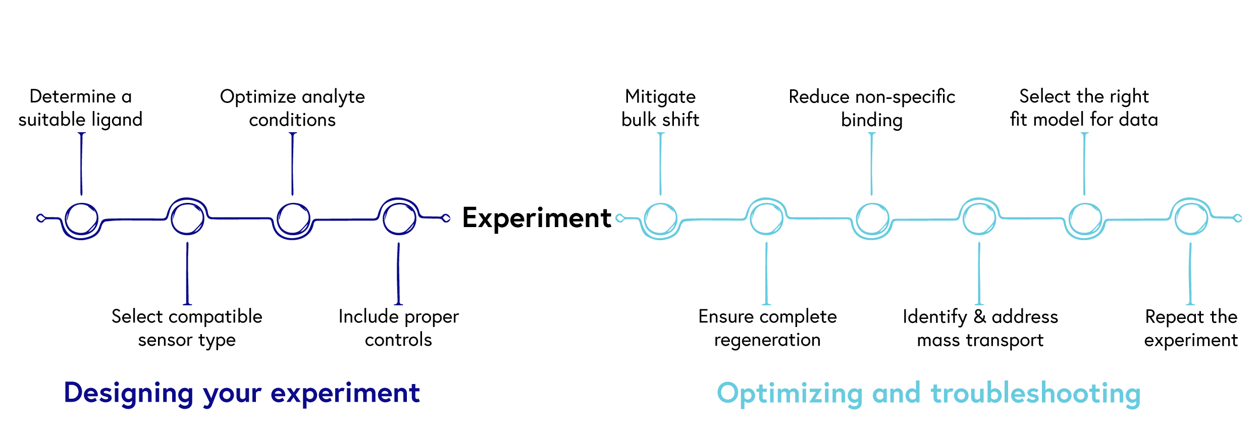
Diligent planning and robust experimental design can save you precious time and resources down the line, while streamlining the path to publication. To help you succeed, we have summarized our top 10 tips for generating robust SPR data (Figure 1).
So what are you waiting for? Let’s get started!
Table of contents
Designing your experiment
1. Determine a suitable ligand
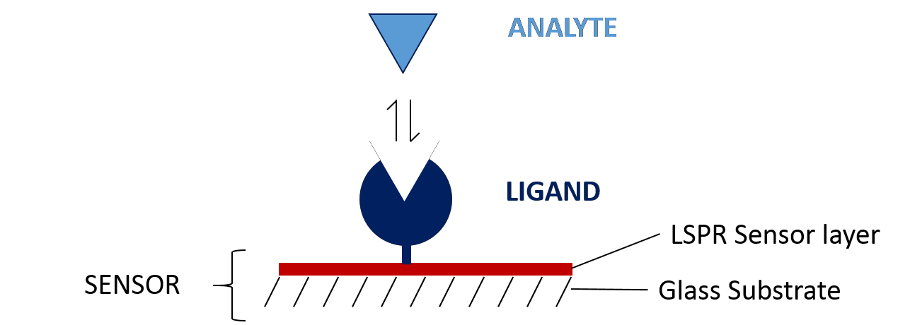
The first step in designing your SPR experiment is to select your two binding partners and decide which to immobilize as the ligand (Figure 2), with the aim of simplifying immobilization, maximizing signal-to-noise ratio and minimizing non-specific binding. Several factors play into this decision, including:
- Size: The smaller binding partner is better suited as the ligand for maximizing the response signal. If there is reason to use the larger binding partner instead, the ligand density on the sensor chip should be increased to amplify the signal.
- Purity: When using carboxyl coupling for immobilization, it is best to use the purest binding partner as the ligand to ensure only the biomolecule of interest binds to the surface. This isn’t as important for a capture immobilization approach.
- Number of binding sites: Binding partners that have two or more binding sites are typically better suited as the ligand. Multivalent analytes will bind to two ligands and provide an artificially low signal compared to the intrinsic affinity of the interaction.
- Tags: In case one of the binding partners is already tagged, consider using it as the ligand. Tags facilitate the immobilization of biomolecules to the surface and often result in higher ligand activity by ensuring proper orientation and binding site accessibility. Ensure compatibility between the tag and your selected sensor chip.
Another parameter to define is ligand concentration. To avoid depletion of analytes at the sensor surface during the association phase, it is generally recommended to use lower ligand densities. You can aim for a higher density for preliminary experiments in case of low surface activity and readjust later if needed.
2. Select compatible sensor type
Now that you have selected your ligand, it’s time to determine the most suitable sensor type for your application. This is largely dependent on the immobilization strategy of the ligand, which is determined by its characteristics. Is it tagged or untagged? Does it have any functional groups? Is it an IgG based antibody? Is it a lipid or a protein reconstituted into a liposome?
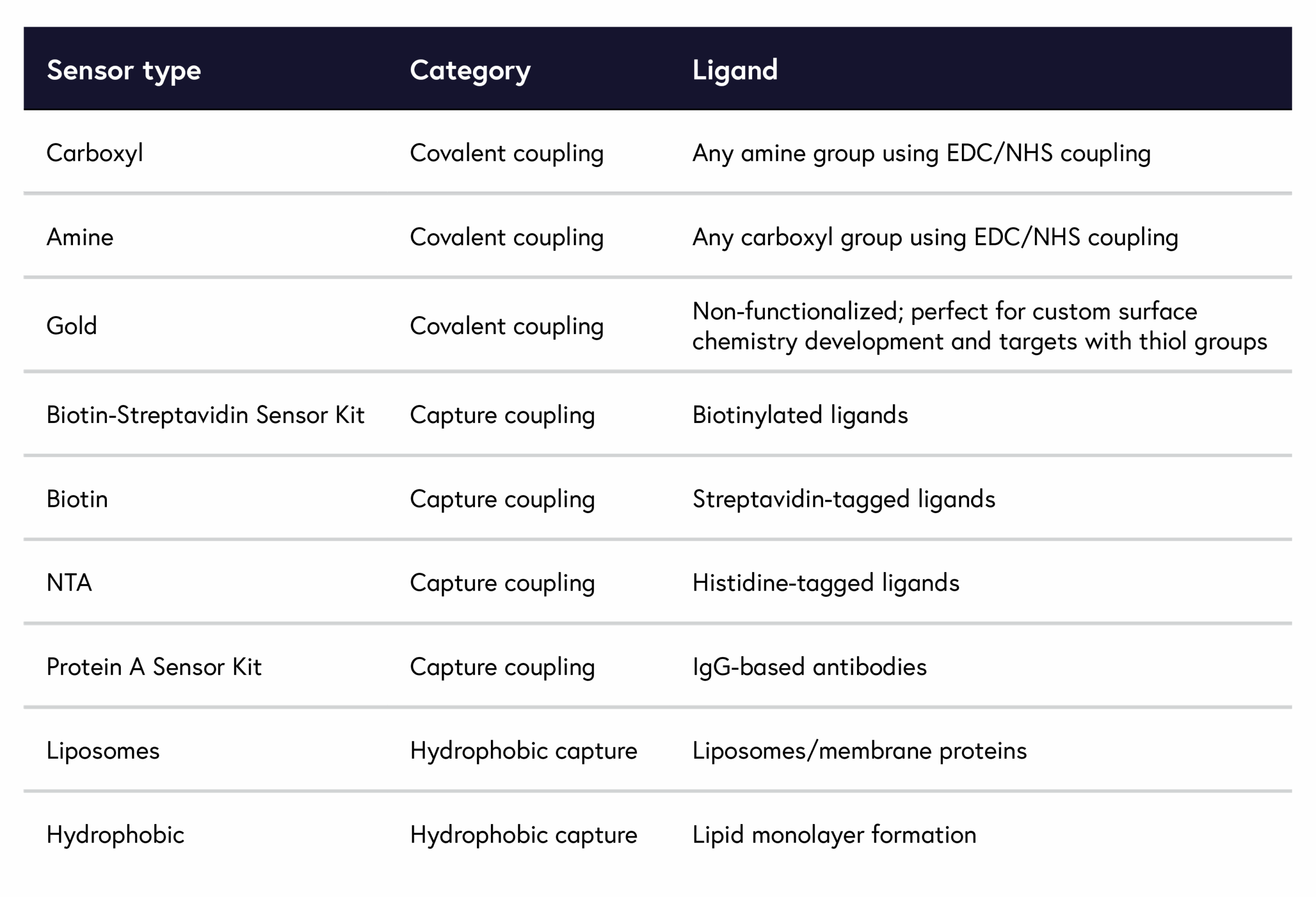
For a broad overview of which sensor to use for your application, refer to Table 1. Keep in mind that there may be more than one possible sensor chemistry for your ligand, each of which offers different benefits that impact immobilization levels and non-specific binding. For instance, a histidine-tagged protein can be paired with both a carboxyl and NTA sensor.
Table 1: Summary of sensors suitable for each ligand characteristics.
3. Optimize analyte conditions
To calculate kinetics with a high degree of confidence, a well-prepared dilution series of your analyte is integral as both the experimentally determined association rate constants (M-1s-1) and the affinity constants (M-1) are dependent on the analyte concentrations.
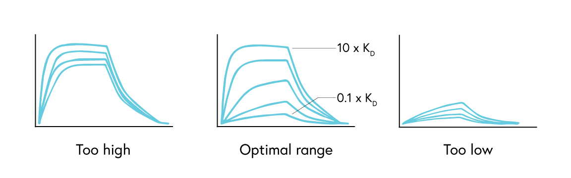
For kinetics analysis, use a minimum of 3, or ideally 5, concentrations between 0.1 to 10 times the expected KD value of the interaction to ensure each resulting curve is evenly spaced over the sensorgram (Figure 3). In cases where the expected KD is unknown, start at a low nM concentration and increase the concentration until a binding response is observed.
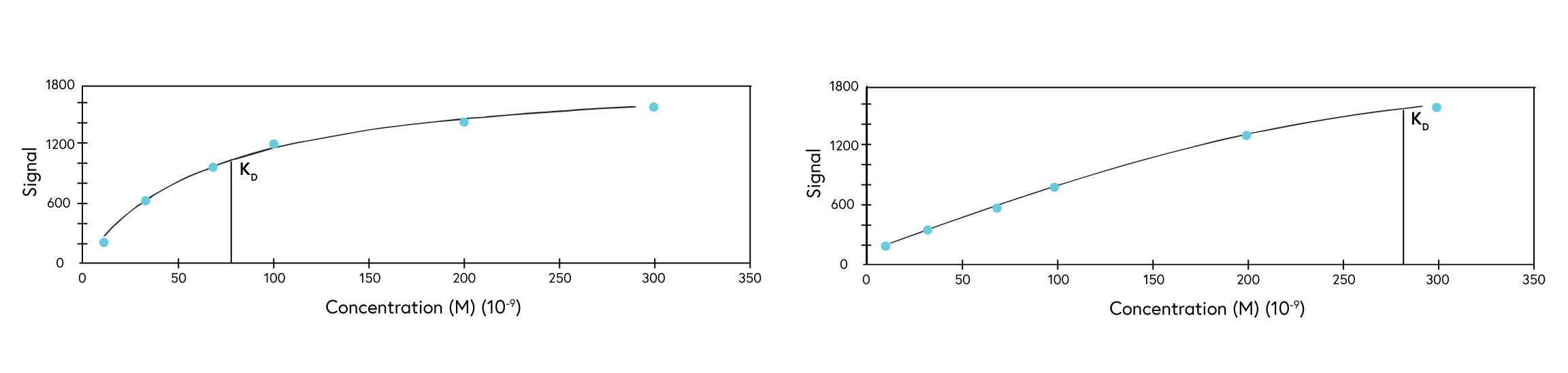
If observing an interaction where steady state is reached very quickly, full kinetics may not be possible to calculate. In this case, perform an affinity analysis by obtaining a single experimental data point from 8 to 10 analyte concentrations. This provides sufficient data to plot the average response versus concentration plot, from which the KD value can be confidently determined (Figure 4). If the reported KD value is higher than half of the highest analyte concentration sampled, repeat the experiment with higher concentrations of analyte samples.
To ensure accurate preparation of your concentration series, opt for a serial dilution approach to avoid errors from repeatedly changing pipettes and volumes between dilution steps.
4. Include proper controls
The last step in designing your experiment is determining proper positive and negative controls and including them in your assays. Using a multi-channel instrument with reference channel subtraction can simplify data correction by compensating for bulk refractive index differences between flow buffer and analyte sample, and discriminating specific from non-specific binding.
You’re now ready to run your first assay!
Optimizing and troubleshooting
Once you have your preliminary data, study it for evidence of artifacts such as bulk shifts, non-specific binding, and mass transport effects. Make sure you do this step before data correction, as artifacts are easier to detect in raw data. In looking for signs of incomplete regeneration and poor data fit, we’ve provided some tips in the sections below.
5. Mitigate bulk shift
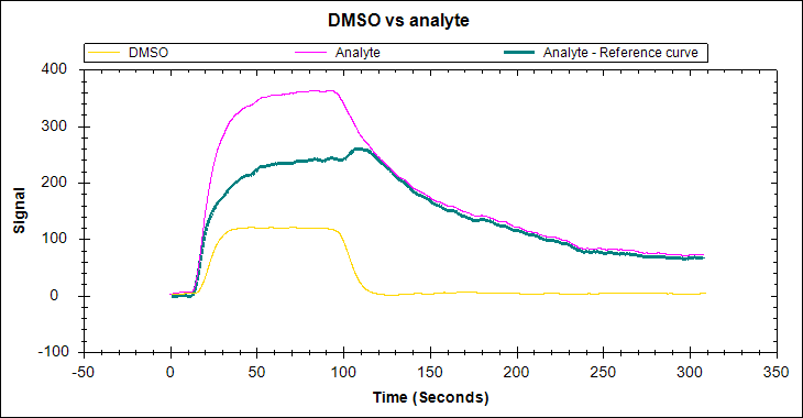
Bulk shift, or solvent effect, occurs as a result of a difference between the refractive index (RI) of the analyte solution and running buffer. This will create a tell-tale ‘square’ shape in your sensorgram due to a large, rapid response change at the start and end of the injection (Figure 5). The shifts may be positive or negative, depending on the RI difference detected.
While the presence of bulk shift does not change the inherent kinetics of the binding partners, it complicates the differentiation of small binding-induced responses and other interactions with rapid kinetics from a high refractive index background. It is therefore crucial to identify and mitigate bulk shifts. While a corrected response can be obtained through reference subtraction. the correction may not always adequately account for the bulk effect. It is, therefore, best to match the components of the analyte buffer to the running buffer, or to avoid buffer components that may cause this effect.
The table below provides recommendations for buffer components that can cause bulk shift, yet cannot be omitted as they stabilize/solubilize the analyte or ligand molecules in solution.
Table 2: Recommendations to reduce bulk shift for common buffer components.
6. Ensure complete regeneration
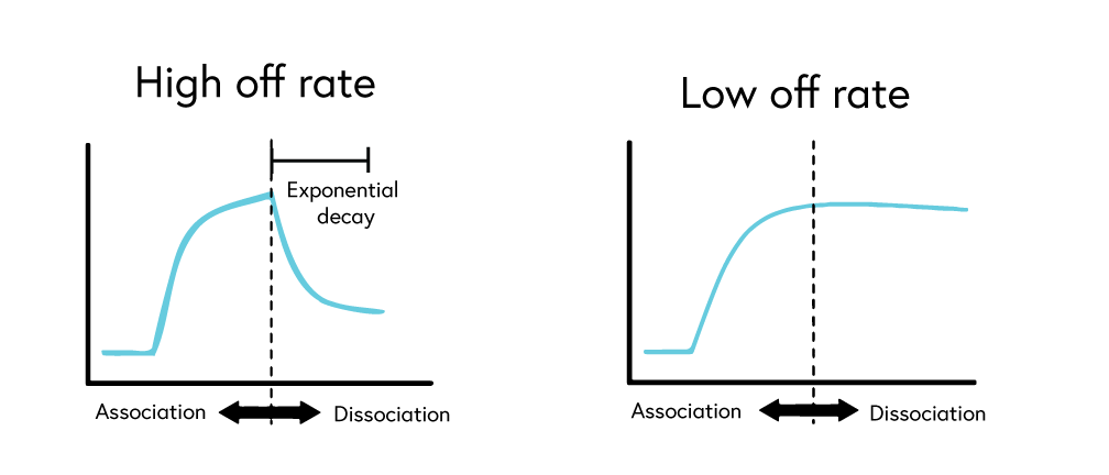
To accurately determine binding constants, complete dissociation of the analyte-ligand complexes is required between each concentration of your analyte. While binding systems with high off rates may fully dissociate from the surface on their own, many systems, such as those with low off rates, require a regeneration step to ensure complete stripping of bound analytes from the ligand.
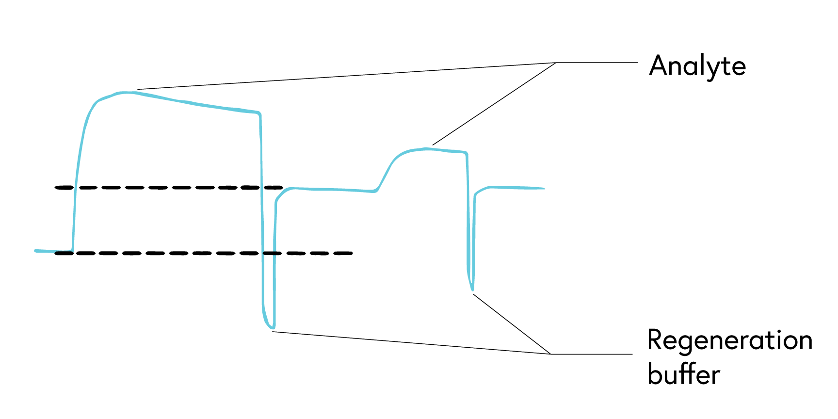
If your system has a low off rate (Figure 6) or shows evidence of incomplete regeneration (Figure 7), the following steps can help to optimize your regeneration step:
- Select a regeneration solution different from the running buffer to efficiently strip the analyte from the ligand.
- Condition the ligand surface prior to injecting analyte by performing 1 to 3 injections of regeneration buffer on the sensor chip.
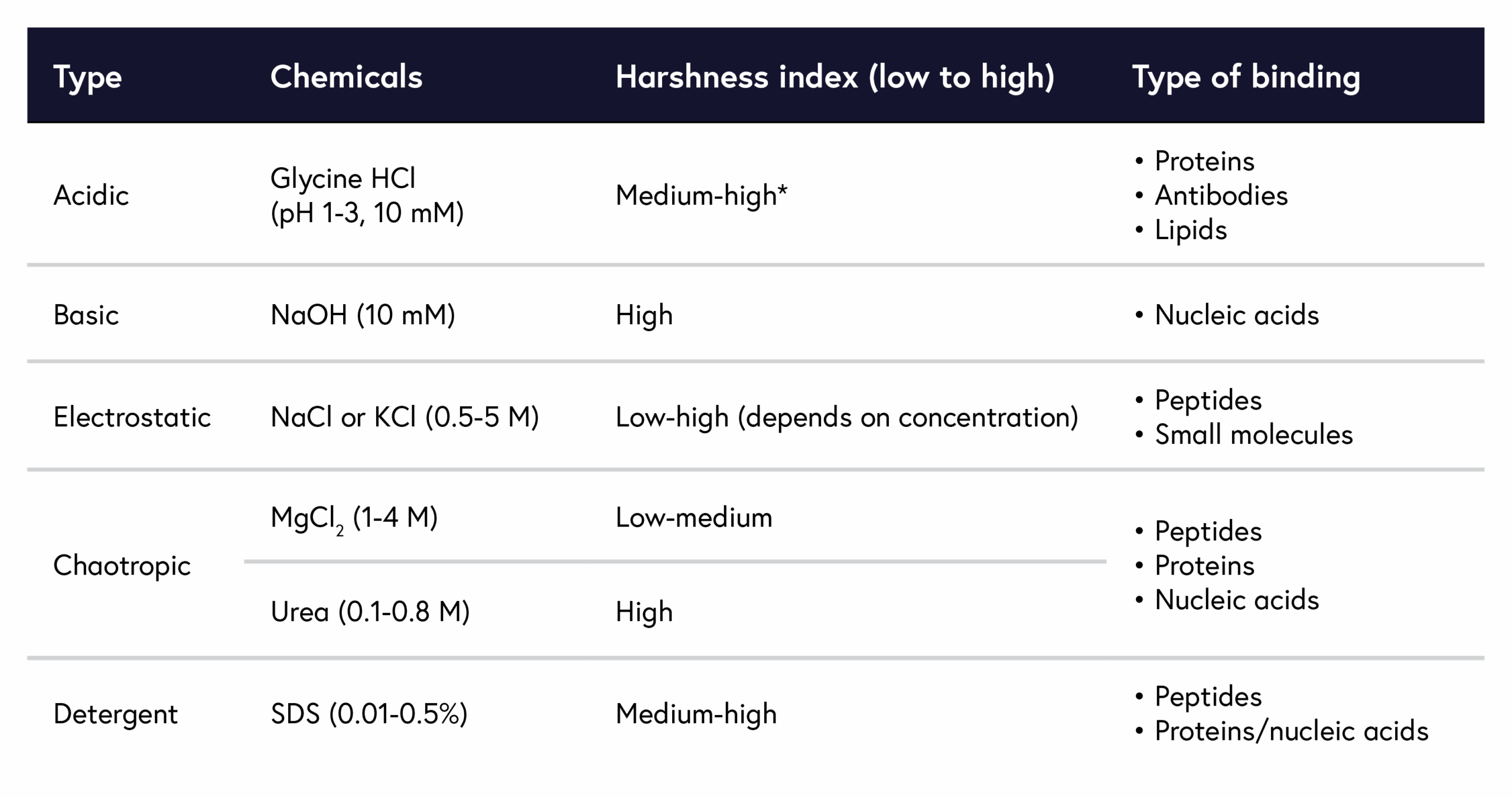
- Formulate a suitable regeneration solution based on your experimental parameters (Table 3).
- Use short contact times to minimize ligand damage (flow rates 100-150 µL/min).
- Include a positive control to verify the analyte response is unaffected by regeneration.
- Ligand re-immobilization may be required after each regeneration step for some sensor chemistries, where the regeneration buffer results in the removal of both ligand and analyte (ex. Imidazole removes histidine-tagged ligand-analyte complexes from the NTA sensor surface).
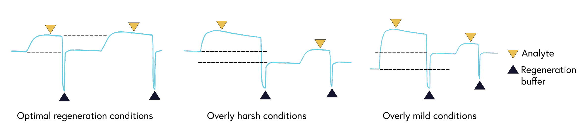
It is critical to choose a regeneration buffer harsh enough to remove all of the analyte, but mild enough to not damage ligand functionality. Begin regeneration scouting by starting with the mildest conditions and progressively increasing the intensity until the surface is completely regenerated. To guide you with finding the optimal condition, we have shown examples of binding curves for optimal regeneration buffers versus overly harsh or overly mild ones (Figure 8).
Table 3: Common regeneration buffers based on type of analyte-ligand bond.
7. Reduce non-specific binding
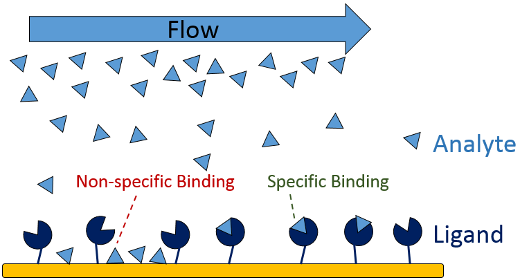
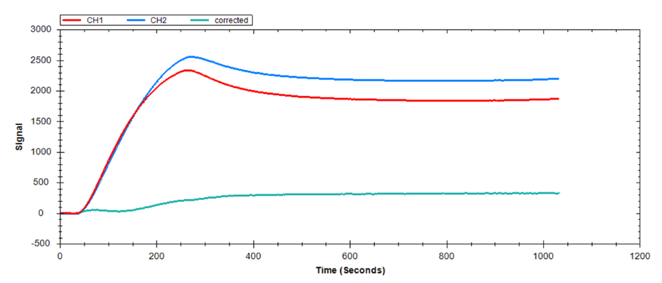
Non-specific binding (NSB) occurs when the analyte interacts with non-target sites on the sensor surface or the immobilized ligand (Figure 9), inflating the measured RU and skewing calculations. Determine whether NBS is present in your binding system by running a high concentration of analyte over a bare sensor with no immobilized ligand as a preliminary test.
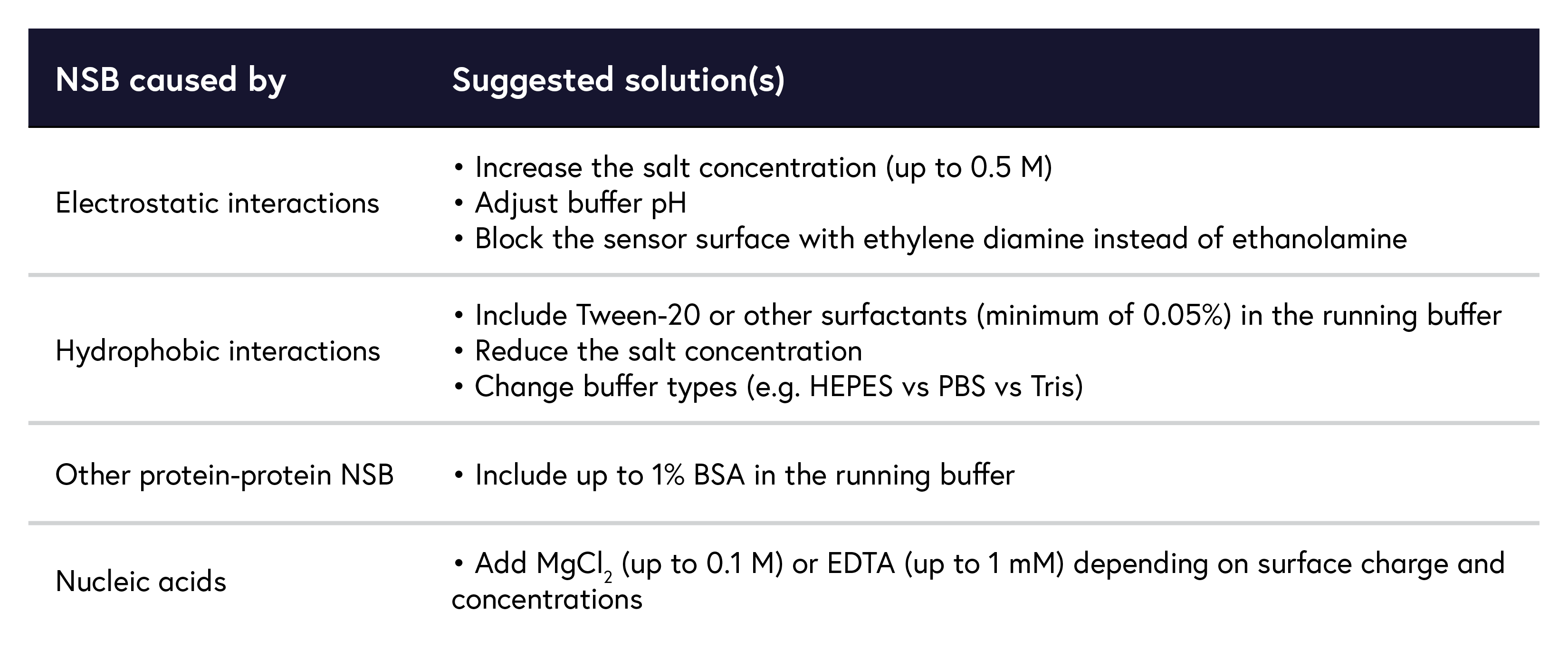
If NSB is observed (Figure 10), there are several approaches you can use to mitigate these interactions. Table 4 lists the most common sources of NSB and their suggested solutions. In cases where NSB cannot be completely eliminated but accounts for <10% of your signal, correct your data by subtracting the NSB signal from the specific binding signal.
Table 4: Common sources of NSB with suggested solutions.
To address NSB, the following approaches may be taken:
- Adjust buffer pH: The pH of the running and analyte buffers can impact NSB by affecting the overall charge of the analyte. A positively-charged analyte will non-specifically interact with a negatively charged sensor surface. In this case, adjust the pH to the isoelectric point of your protein, or neutralize the surface of the sensor.
- Use protein blocking additives: If using a protein analyte, add bovine serum albumin (BSA) to your buffer and sample solutions during analyte runs only. Using during ligand immobilization will result in BSA binding to the sensor surface. As a globular protein with domains of varying charge densities, BSA shields molecules from non-specific interactions. BSA is usually used at a concentration of 1%, but can vary from experiment to experiment.
- Add non-ionic surfactants: If NSB is occurring due to hydrophobic interactions in your system, it may be beneficial to use non-ionic surfactants such as Tween 20. Low concentrations of this mild detergent disrupt hydrophobic interactions between the analyte and sensor surface.
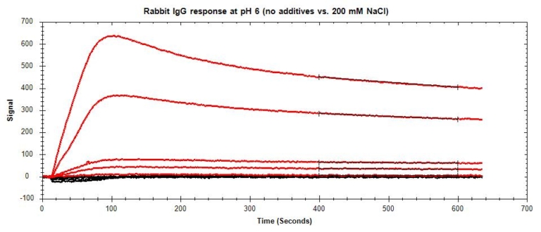
- Increase salt concentration: If NSB is occurring primarily due to charge-based interactions, increase salt concentrations in your buffer to reduce these interactions by shielding your analyte. Salts such as NaCl can be used at varying concentrations to prevent charged proteins from interacting with other charged surfaces, including the sensor surface.
- Switch ligands: When working with negatively charged carboxyl or NTA sensors, use the more negatively charged molecule as the analyte. If you are unsure which molecule will have the least NSB, run a non-specific binding test on each.
- Change sensor chemistry: Avoid opposite charges between your sensor surface and analyte, which leads to non-specific interactions.
8. Identify and address mass transport
When the diffusion rate of the analyte from the bulk solution to the sensor chip surface is slower than the association rate constant (ka) of the binding system, the binding kinetics becomes mass transport limited and may skew the resulting data. Mass transport limitations are most common for fast binding reactions, low analyte concentrations, poorly diffusing analyte, and lower flow rates. It’s important to identify and properly address this phenomenon to ensure data reliability.
To identify mass transport effects:
- Examine the binding curve: A linear association phase with a lack of curvature signals mass transport limitations (Figure 12).
- Conduct a flow rate experiment: Run your assay using a few different flow rates. If the ka decreases at lower flow rates, the interaction is mass transport limited.
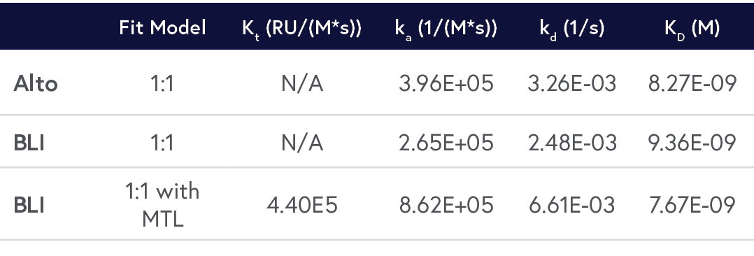
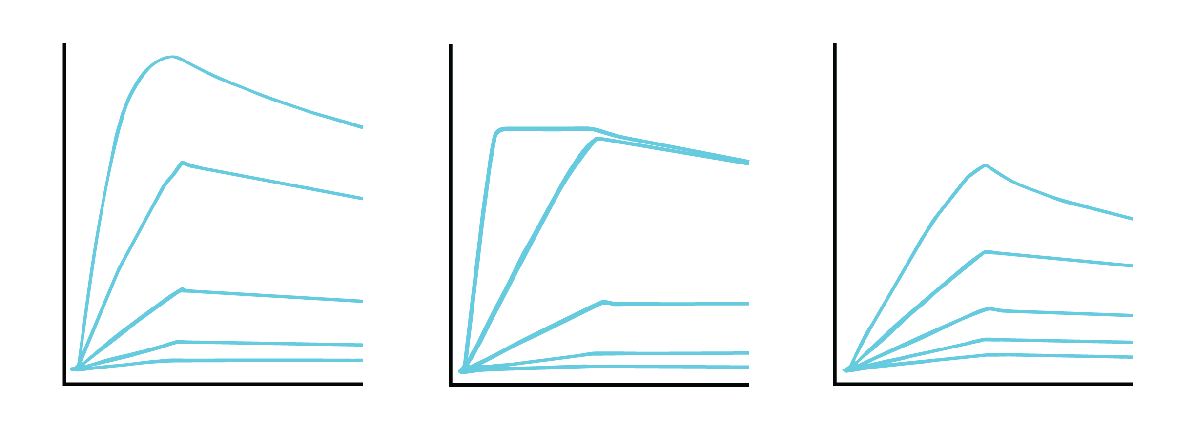
- Compare data fits: Fit your data using two different Langmuir models available in TraceDrawer. Fitting with both the 1:1 Langmuir model and the 1:1 Langmuir mass transport corrected model will identify if your interaction is mass transport limited by showing a lower ka for the 1:1 Langmuir model.
If you find your data to be mass transport limited, there are several approaches you can take:
- Increase flow rate: Increasing flow rate will increase the rate of diffusion by delivering the analyte to the immobilized ligand faster, without affecting the kinetic data. This can also be achieved by increasing the analyte concentration. The trade-off is that the analyte might not have enough time in the association phase.
- Decrease ligand density: Decreasing ligand density on the sensor will mitigate diffusion-limited effects by limiting possible interaction sites for analytes to bind. This is especially key for fast binding analytes. The trade-off is a decrease in the max signal at saturation (Rmax), yielding noisier data.
- Use a mass transport corrected model: Use a fitting model that includes mass transport in the overall reaction equations. Most kinetic processing software include this model as an option when fitting data, including TraceDrawer. The only trade-off is that data fitting may take a bit longer.
9. Select the right fit model for data
Now that you have your results, it’s time to analyze and fit your data. For many scientists, SPR data analysis can be tedious and puzzling. Our intuitive, user-friendly and robust SPR data analysis software will guide you through the experimental procedure and data analysis, providing several fit models for different needs.
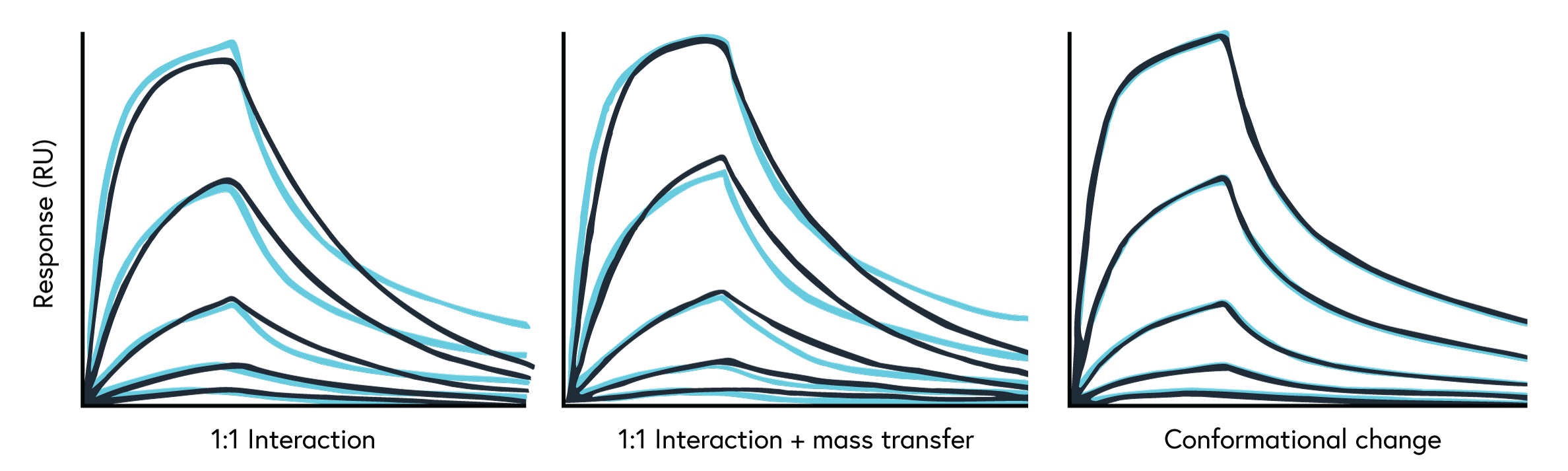
The first order of business is fitting your data with the simplest binding model, a 1:1 global fit. If that fit isn’t ideal, it’s important to understand why your data doesn’t fit well instead of trying to figure out how you can make it fit better with software. To evaluate the quality and confidence of the data fit, consider the following:
- Visual evaluation: The fits should approximate the actual data. Significant departures across all analyte injections indicate a poor fit or the presence of artifacts.
- Standard error: The standard error indicates how well that value is defined (i.e. how well the KD is fit). Ideally, this value should be a minimum of one or two orders of magnitude lower than the value.
- Residuals: A good fit has residuals that are very low compared to the intensity of the binding curves, and randomly scattered in a narrow band around zero.
If there is experimental evidence suggesting an alternative binding model is present in your binding system, apply the relevant fit model. The following may signal you to use a fit model other than a simple 1:1 global fit, all of which are provided on our SPR software:
- Mass transport limited binding systems
- Bivalent binding systems
- Modulating interactions (i.e. cooperative binding)
10. Repeat the experiment
The benchmark of high-quality scientific data is reproducibility. Run your experiment multiple times to corroborate your data precision, get a standard deviation for your kinetic results, and ultimately present more credible data. Once you’re confident in your results, it’s time to publish your article and share your findings with the scientific community. Here are two guides to help you in the process: Technical Guide: Expert Tips on Publishing Your SPR Data; and 5 Tips on Getting Published in a High-Impact Journal.
These 10 tips should help you design, troubleshoot, and optimize your assay to ultimately get high-quality SPR data. Our next-gen platforms OpenSPR™ and Alto™ have been designed to take the complexity out of SPR by providing a seamless user experience from assay design to data analysis. Learn how to leverage our high-throughput, automated platforms to streamline your research workflow by contacting us today!