Trying to get your research manuscript accepted faster?
Publishing your work is an incredibly rewarding feat and is integral to the career of an academic researcher. We previously shared some great tips to help you get published in a high-impact journal. Recognizing the importance of presenting reliable data, this blog focuses specifically on how to strongly present surface plasmon resonance (SPR) data to help you get published.
With more journal reviewers asking for quantitative binding kinetics data, many researchers choose to use surface plasmon resonance (SPR) to study their molecular interactions. This is because SPR provides label-free, publication-quality kinetics data in real-time. Furthermore, the OpenSPR™ is an SPR solution that is affordable, user-friendly and low maintenance.
Presenting data that is reliable and backed by evidence is crucial in getting published, regardless of the technique. Not only does this show your credibility, but it also helps your research manuscript get accepted faster. Submitting reliable data helps you spend less time emailing your editor and more time on what’s most important – making your next big discovery.
Our latest blog post offers tips on evaluating your binding curves and what data to include to ensure your SPR data is correctly presented and properly documented.
Evaluating your binding curves
Before looking at an ideal binding curve, let’s look at some common artefacts (i.e. mass transport effects, non-specific binding, bulk shifts), found in an SPR binding curve. Once identified, you can correct them. If you are ever unsure if your SPR data contains artefacts, don’t worry – you’re not alone. Anyone with an OpenSPR™ has access to our Customer Success Scientists (CSS) to look over your data with you and help you produce publication-quality data.
Mass transport effects
Mass transport is defined as the transport of analyte from its bulk solution to the sensor chip surface. When this transport is slower than the association rate constant (ka) of the binding system, the binding kinetics will be mass transport limited. This can lead to inaccurate measurements. This effect can arise from a number of conditions, including low analyte concentration, using a poorly diffusing analyte, high ligand density and low flow rate.
Mass transport effects can sometimes be identified as an association phase with a lack of curvature. If you are observing this trend, consider reducing your ligand density, increasing your analyte concentration and flow rate. Some mass transport effects can be accounted for when fitting your data as well. However, it is recommended to take steps to avoid mass transport effects first.
Non-specific binding
Non-specific binding (NSB) occurs when the analyte interacts with the sensor surface, as opposed to the ligand. This creates a false positive. You can test your binding system for NSB by running a non-specific binding test. This is when you run a high concentration of analyte over a sensor with no ligand immobilized to see how your analyte interacts with the sensor.
It is essential to run an NSB test for every experiment to ensure the data is indeed representing the actual binding of your analyte to the ligand! There are a number of experimental methods to reduce non-specific binding, such as increasing salt concentration, adjusting buffer pH, and adding surfactants. For more information, read our technical guide on non-specific binding.
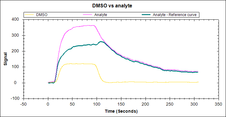
Tip: If you’re using a 2-channel OpenSPR™, you can also identify non-specific binding by a large signal increase in your reference channel (which should not contain your ligand) during your analyte injections.
Bulk shifts
Bulk shifts occur as the result of a difference in the refractive index between your analyte buffer and your running buffer. This will create a tell-tale ‘square’ shape in your binding curve due to the large, rapid response changes at the start and end of the injection. If you observe this trend, it is likely due to a difference between your running buffer and your analyte buffer. Note that it can be sometimes challenging to distinguish binding and bulk shifts for small molecules and other interactions with rapid kinetics; for experts’ help contact our Customer Sucess team!
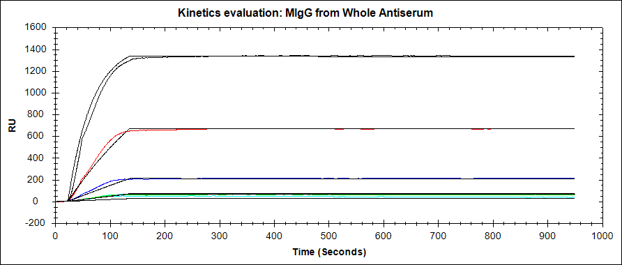
An ideal SPR binding curve
As you can expect, an ideal SPR binding curve is free of the artefacts listed above. The association phase should follow a single exponential, with curvature before the injection is complete (at least for the highest concentration levels). The curve should round out and become relatively flat as the interaction approaches equilibrium. The disassociation should also follow a single exponential and be long enough to observe a 5% signal decrease.
Improving the credibility of your binding curves
In addition to watching for these common artefacts in your data, here a few more suggestions to prove the reliability of your data:
- Ensure that the ligand is fully regenerated between analyte injections using an appropriate regeneration solution (if necessary).
- As with any analytical technique, perform your binding experiments in duplicate or even triplicate. This way you can get a standard deviation for your kinetic results, comment on the consistency between experiments, and ultimately present more credible data.
- Analyze binding at enough analyte concentrations to properly calculate kinetics. Most SPR experts recommend using 5* separate analyte concentrations.
- In the same vein, your analyte concentrations should be well spaced out. It is recommended to use a concentration range between 0.1x and 10x the expected KD of your interaction if it is known. If your curves are not sufficiently spaced out, it may be because you are targeting the wrong concentration range.
* If performing steady-state affinity analysis, 8-10 separate analyte concentrations should be used. It is also imperative that equilibrium is reached, which is observed by the binding curve flattening out at the end of the association phase.
Presenting your data and showing your work
At this point, you have evaluated your binding curves and concluded that the data is of good quality. Here are some expert tips on how to present your data and what additional data to include so that reviewers can confirm your binding curves are reliable:
- The corrected raw data (analyte binding subtract reference) should be shown with the fits overlaid. If only the raw data is shown, there is no evidence behind how the kinetic constants were calculated! Similarly, if only the fits are shown, there is no way to see if they fit the raw data properly.
- The use of a reference should be explicit. If using a multi-channel instrument with built-in referencing options, this can be as simple as stating that references were taken in real-time, and the corrected data is shown. If using a one-channel instrument, the binding curves from your reference experiment or an NSB test should be available for the reader to observe.
- Your raw data should always be available, at least as supplemental data. This avoids casting doubt on the credibility of the experiment, as another SPR researcher could analyze the data and get the same results.
- Ideally, the conditions and results of your ligand immobilization step should also be included for maximum reproducibility..
- If you believe that your binding mechanism does not follow a standard 1:1 interaction, sufficient evidence must be shown to back this. This could be structural data using a different technique, or a more complex SPR analysis.
- Your experimental discussion should be descriptive enough for someone to repeat your experiment. Some important data points to include are:
- Instrument and sensors used
- Interaction temperature
- Analyte concentrations
- Composition of running buffer, analyte buffer, and regeneration solution
- Immobilization conditions (e.g. ligand concentration, chemistry used, buffer and pH etc.)
- Flow rates used for immobilization, regeneration, and analyte injections
Publish faster with OpenSPR™
At the end of the day, the more information you can include about your SPR experiments, the more credible your data will be. And while evaluating your curves is not always trivial, you’re not alone. Researchers using an OpenSPR™ instrument have access to our team of Customer Success Scientists to help with experiment optimization and data analysis. Think of them as an extension of your lab, helping you succeed with your SPR experiments and getting you ready to publish faster with reliable data.